Example (1) Computing a River with a Confluence

In this example we compute a river that includes a confluence/bifurcation.

Starting iRIC and selecting the solver

On the iRIC opening screen, select [New Project] (Fig. 1).

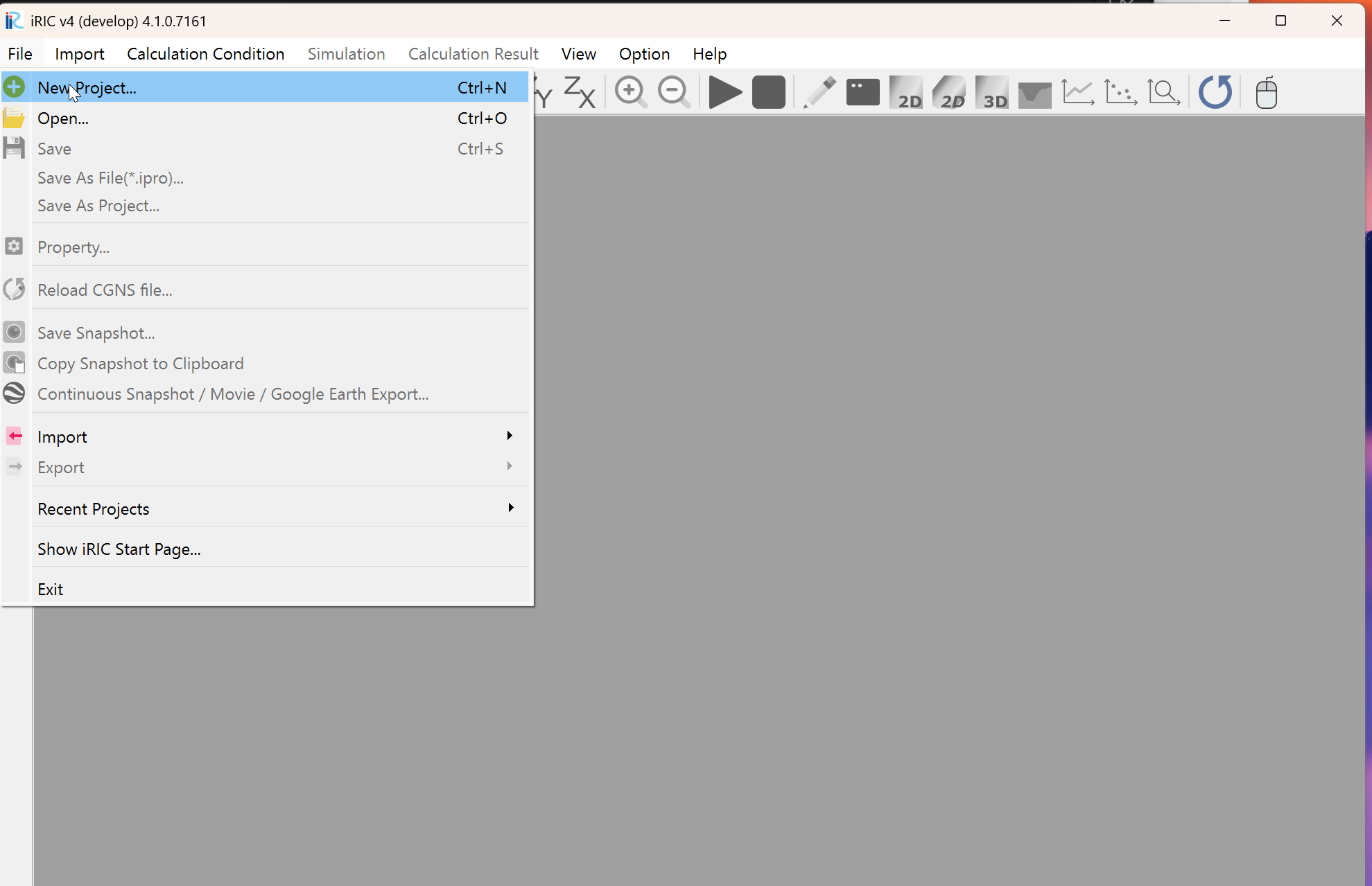
Fig. 1 : New Project

In the solver selection window shown in Fig. 2, select [Cabernet2d] and press [OK].

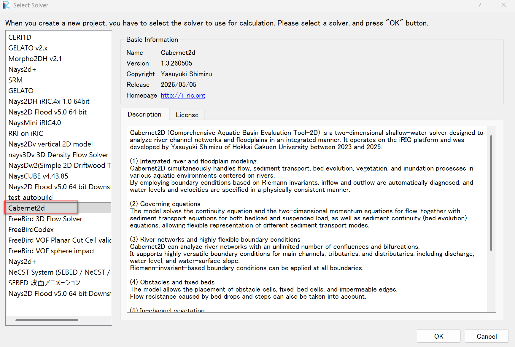
Fig. 2 : Selecting the solver

Creating the computational grid

To set the scale of the current preprocessor view, set a reference line (here, 100 m) following the animation below.

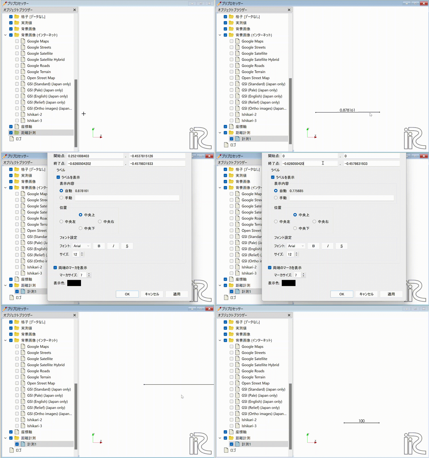
Fig. 3 : Drawing the reference line

From the main menu, choose [Grid] -> [Select Grid Generation Algorithm].

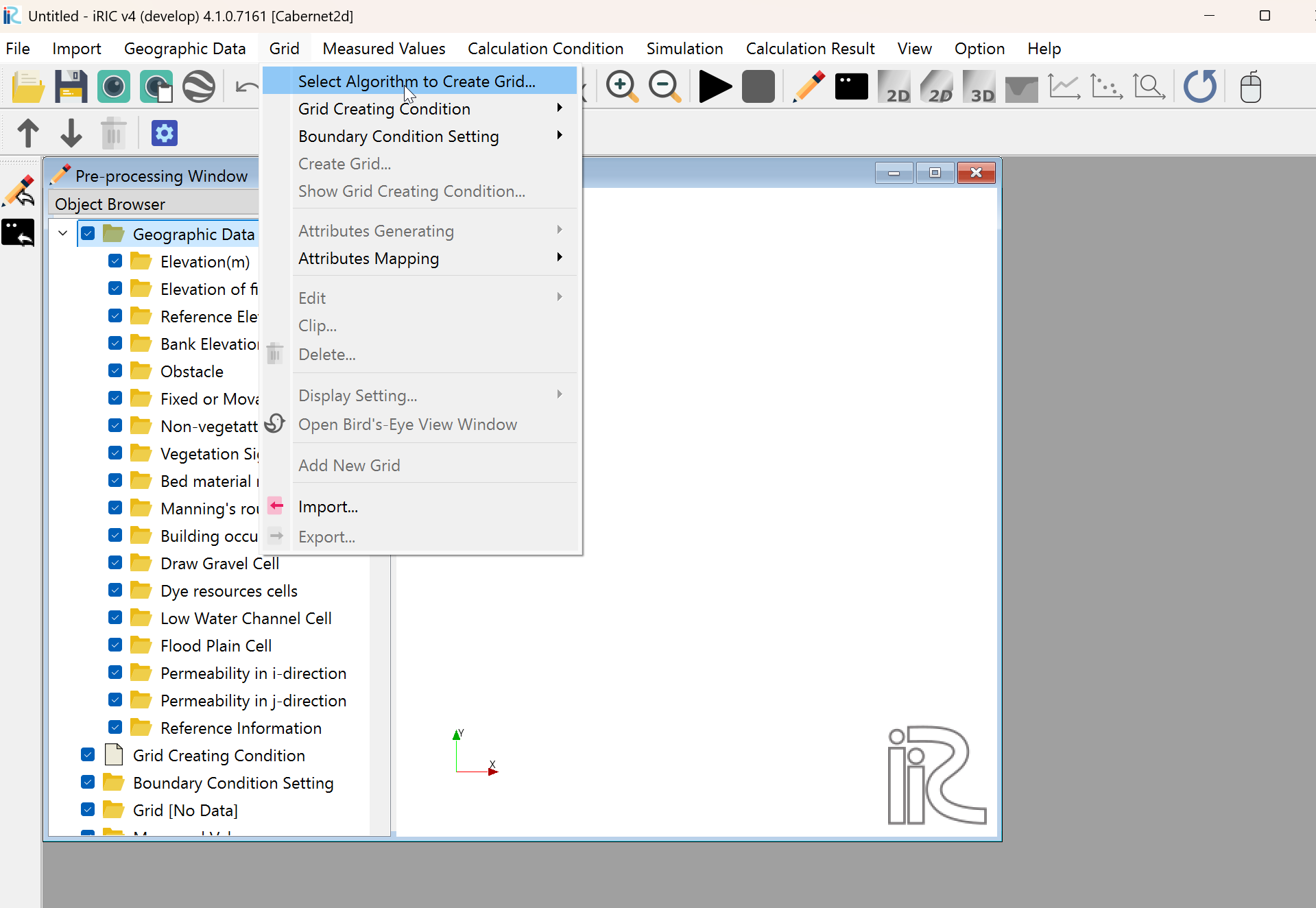
Fig. 4 : Grid generation (1)

In the [Select Grid Generation Algorithm] window, choose [General-purpose grid generation tool] and press [OK].

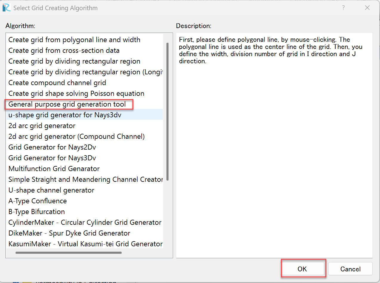
Fig. 5 : Grid generation (2)

A message “Cross-section survey data not found. Please create it yourself.” appears; press [OK].

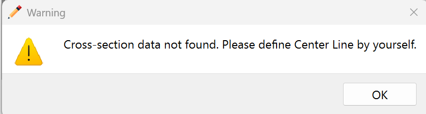
Fig. 6 : Warning dialog (1)

Generate the grid following these steps.

1. Hold down the right mouse button and drag to draw the channel center line, finishing with a double-click.

2. Right-click on the drawn reference line and select [Generate Left/Right Bank Lines (B)].

3. Enter the distance (m) from the center line to the left and right banks and press [OK]. (Here, 30 m is used on each side.)

4. Specify the subdivision lines, grid spacing and other conditions.

5. Set the land area between the upstream main channel and the tributary as an obstacle.

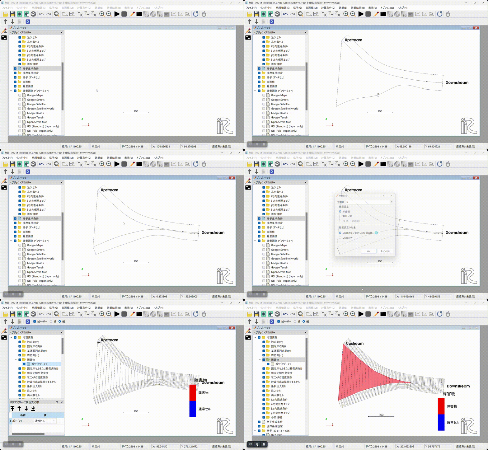
Fig. 7 : Grid generation

Setting boundary and calculation conditions

Set the boundary conditions for the inflow and outflow sections.

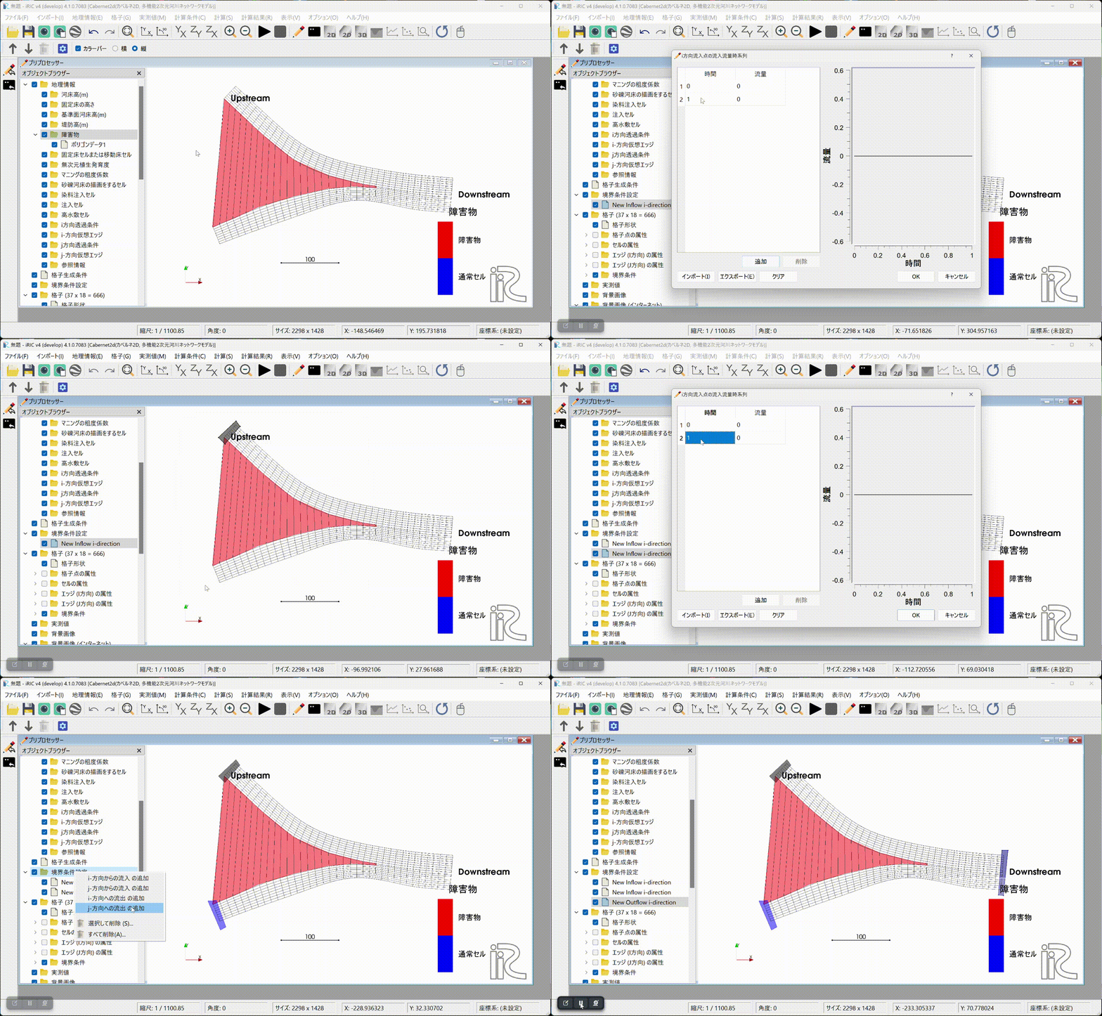
Fig. 8 : Setting boundary conditions

Map the obstacle information and the boundary condition information onto the computational grid.

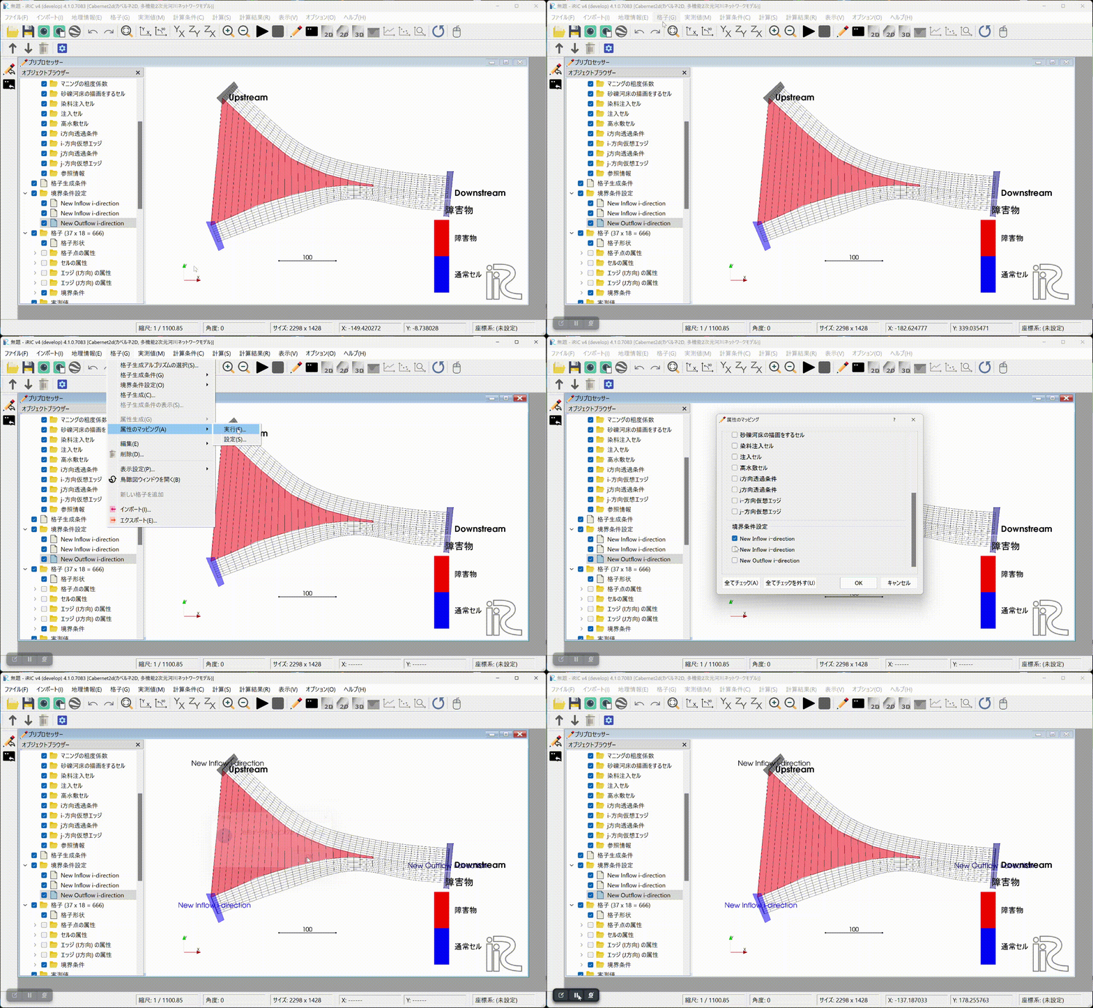
Fig. 9 : Running the mapping

Set the calculation conditions.

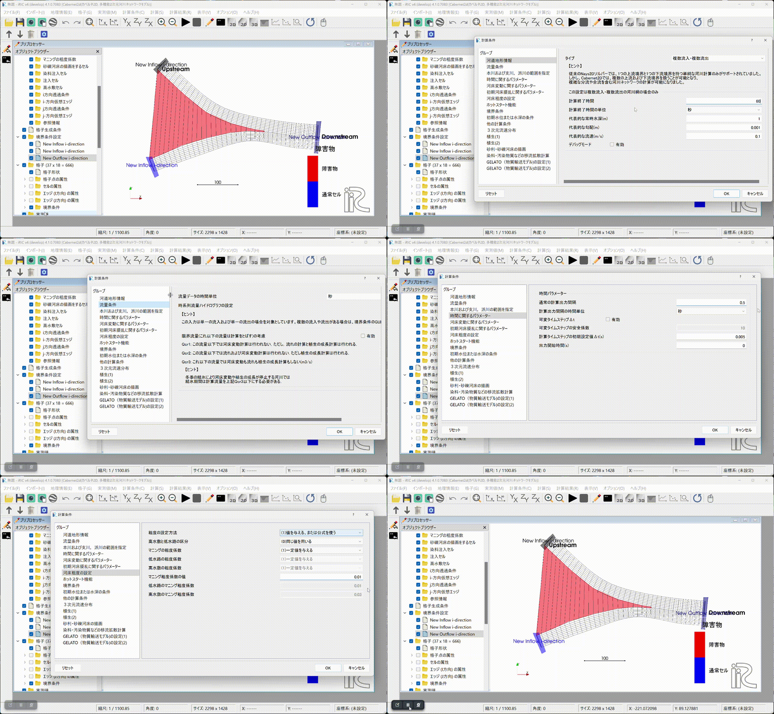
Fig. 10 : Setting the calculation conditions

Running the computation and displaying the results

Run the computation. The first time you run it, you will be asked whether to save the project. Here, we save the project with a new name in a new folder. If you prefer, you can also save the project as a compressed .ipro file.

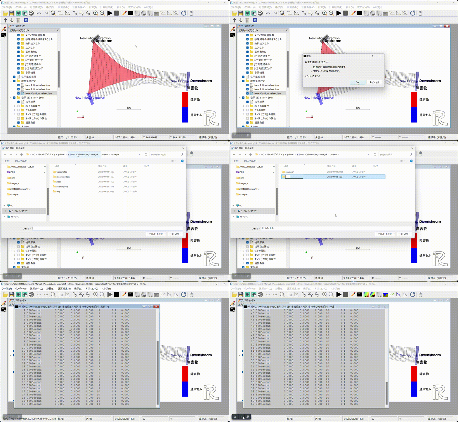
Fig. 11 : Running the computation

Displaying the results (1). Open the 2D post-processing window to display the computation results. In this example we ran a 60-second computation, but at 60 seconds the flow does not appear to have reached the downstream end yet.

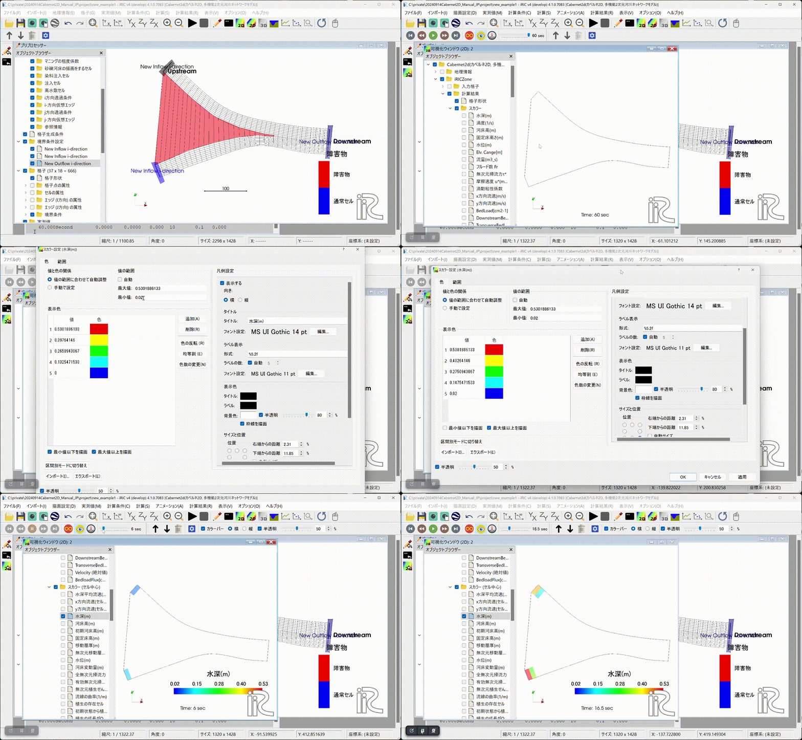
Fig. 12 : Displaying the results (1)

Set the computation time to 600 seconds. Change the boundary and calculation conditions accordingly, run the mapping again, re-run the computation, and display the results in the post-processing window.

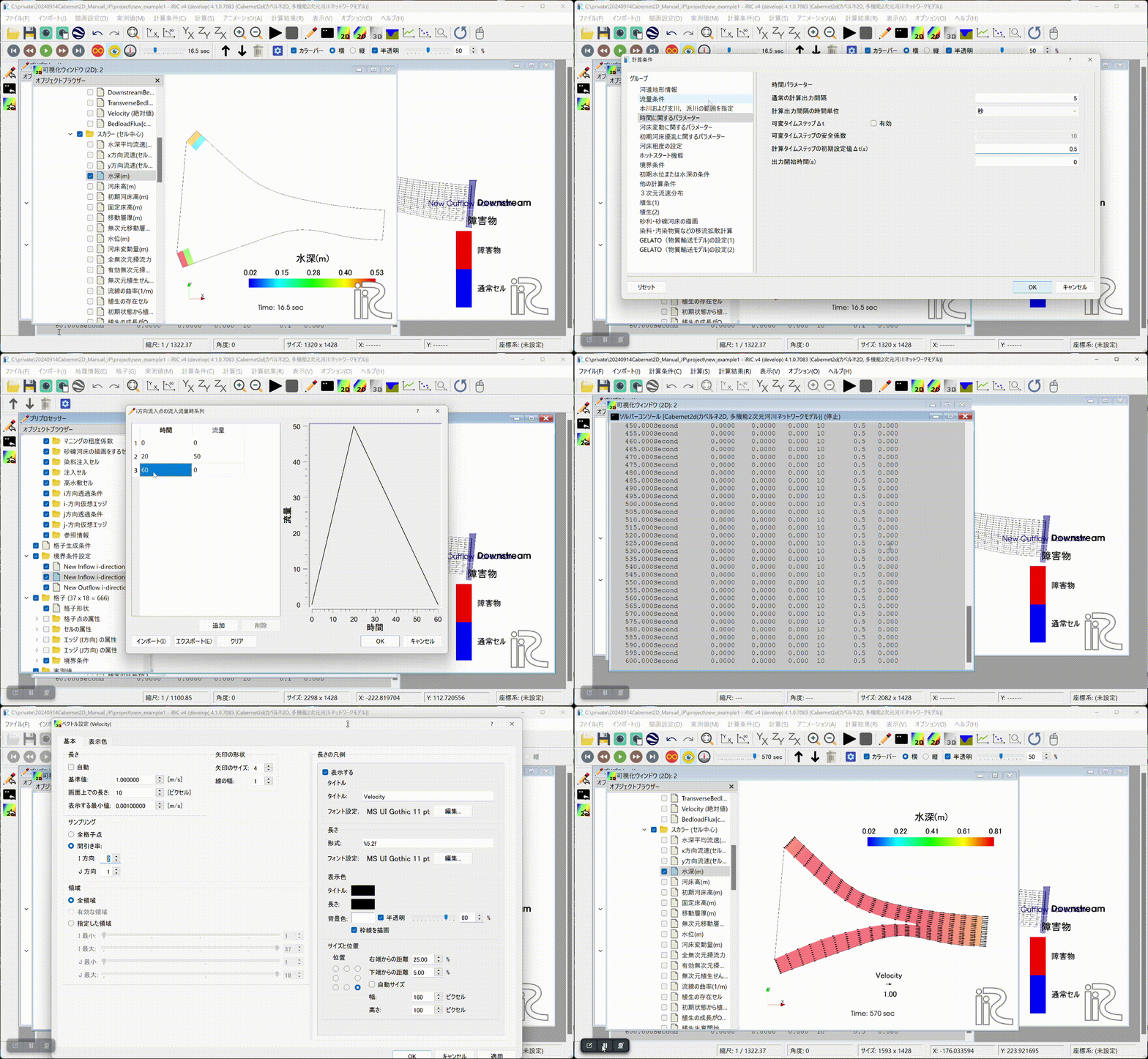
Fig. 13 : Changing conditions, re-running, and displaying the results (2)

Create a discharge hydrograph, longitudinal water-level profile, and other plots, and build an animation from them.

Fig. 14 : Creating plots and building an animation

The resulting animation is shown below.

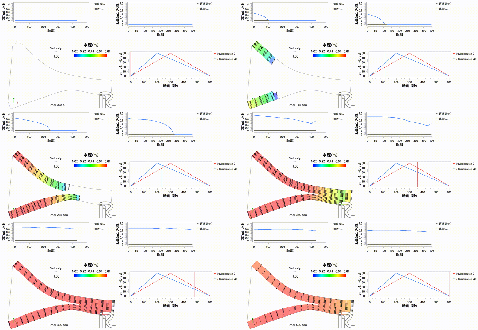
Fig. 15 : Animation of the computation results

The above results are also published on YouTube.